Mapping the climate similarity of U.S. cities

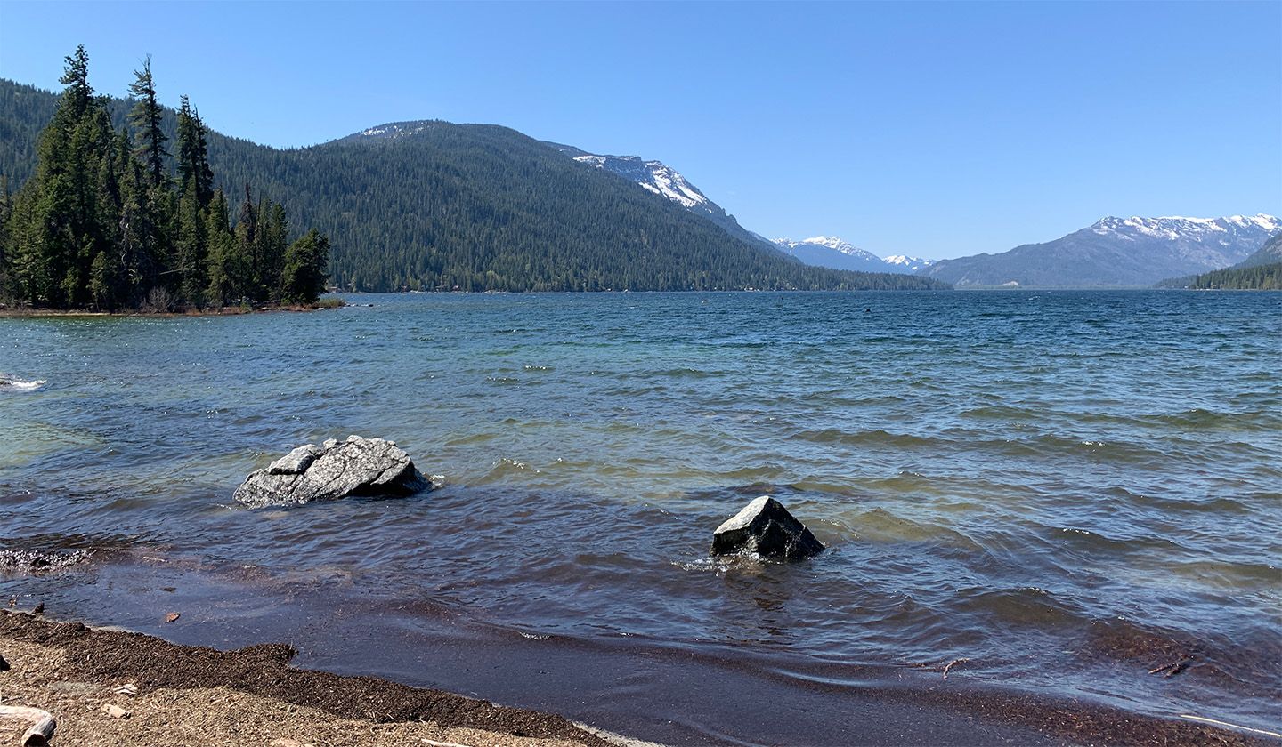
Recently I was standing on the shore of Lake Wenatchee in Washington and considering how similar it felt to Odell Lake, 300 miles south in Oregon. Both are glacier-carved lakes on the east slopes of the Cascade mountains, so climactically they should be similar. Yet there are differences in the species of trees and other flora that can be found at each; Odell is dominated by true Firs while Wenatchee has a mix of Douglas Fir and Ponderosa Pine.

Climate is the primary factor in determining what sort of plants grow where. The Köppen climate classification system—which groups areas by climate similarity—is based at a high level on vegetation type. The two are interrelated: areas with similar climate should also have similar vegetation.

Rather than relying on broad proxies such as vegetation type to classify climate similarity, I wanted to experiment with quantifying climate similarity through metrics directly. Metrics such as precipitation, temperature, dewpoint, and solar radiation.

Using monthly 30-year normals for each of these metrics, I compared how similar a specific place—in this case each city from a set of 50 reference cities—is to everywhere else in the United States. Here’s the result, followed by more details on how I made it:

Climate similarity of reference cities to all other places in the U.S.

Quantifying climate similarity

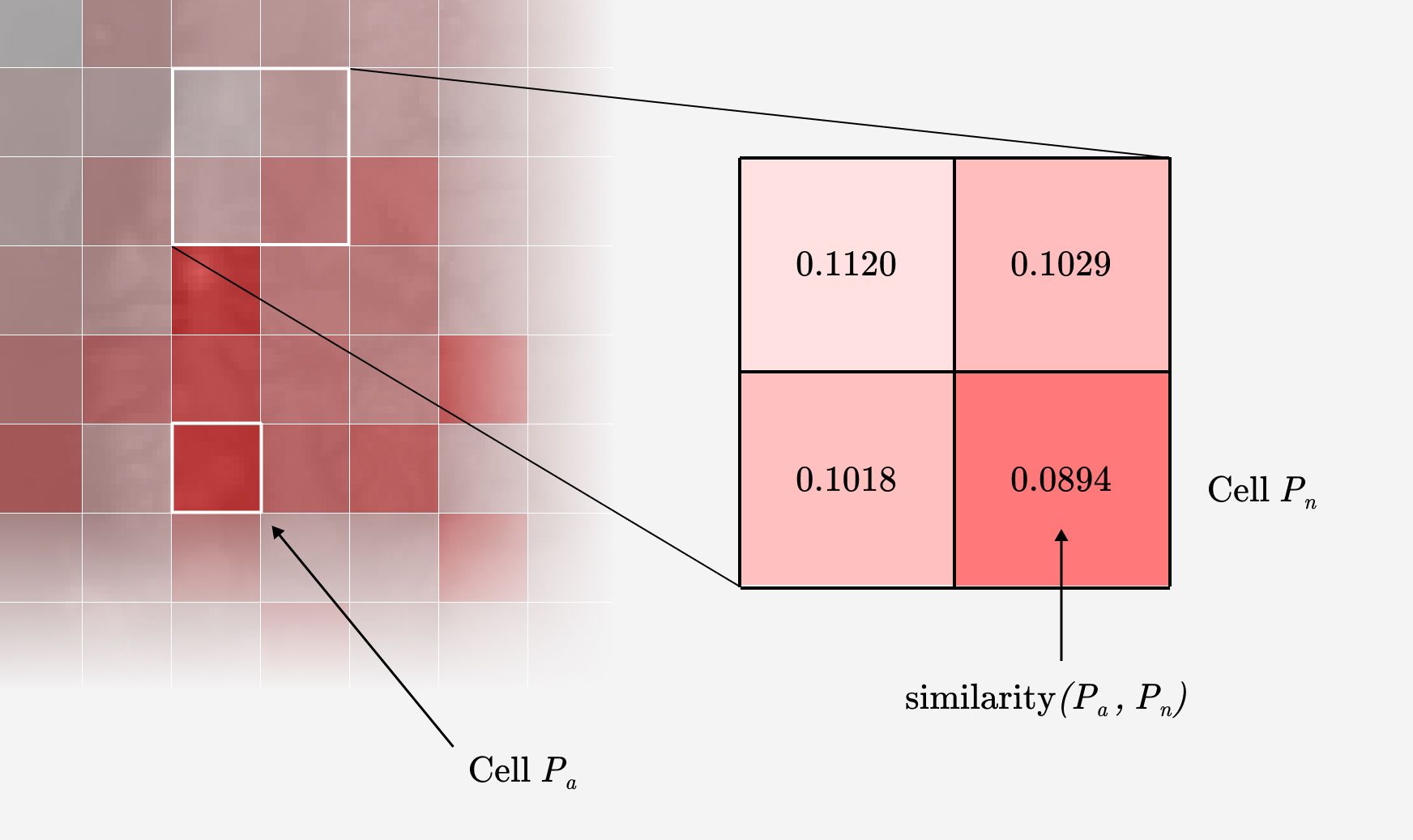
Here’s the approach I used: suppose you take a grid and placed it over the earth. Then you collect climate metrics for each grid cell. Metrics such as precipitation, max temperature, min temperature, and dewpoint. Each of these metrics are averaged for each of the 12 months. So each cell is represented by a two dimensional array: one dimension is the metric and the other is each month.

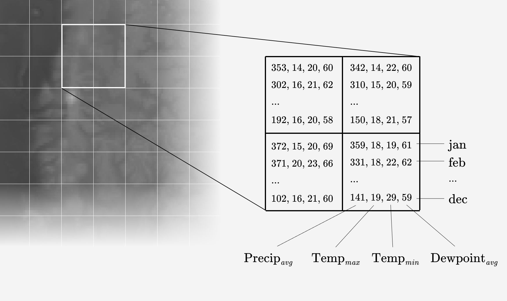
Then you compare a grid cell of interest $P_a$—the coordinates a specific city—with all other grid cells. You put the metrics you’ve collected through a function such as cosine similarity or euclidean distance. These functions take two $n$ dimensional arrays and produce a measurement of the distance between them. So for each grid cell $P_i$ you get a single metric that quantifies that cell’s similarity to the comparison cell $P_a$.

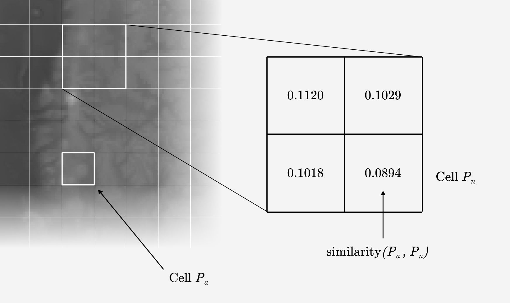
Then you assign a color to the similarity score, creating a map of more and less similar climates.

Sourcing the climate data

I used data from PRISM at Oregon State University. It is delivered in raster format, where each pixel represents a single climate metric for that area.

PRISM provides 30-year normal data for many climate metrics. After some research I decided on using average precipitation, average maximum temperature, average minimum temperature, mean dewpoint temperature, and solar radiation. Each of these 5 metrics is provided for 12 months of the year, resulting in 60 raster layers of data.

Normalization

The next step is to normalize the data. Each metric was recorded in a different unit—such as millimeters or degrees celsius—and therefore had a very different range. Additionally, because the climate of the U.S. is immensely varied, each metric included a number of outliers. These outliers could throw off the final scale of the similarity values, making very different climates appear similar relative to enormously different climates such as Death Valley or the Florida Keys. More on that issue is discussed in the visualization section below.

To solve both of those problems I fit the data to a normal distribution using scikit-learn’s QuantileTransformer. This ensured all the metrics were set to the same range and fit a normal distribution, minimizing the affect of huge outliers.

Calculating similarity

To calculate similarity, I put the 60 normalized climate metrics for a reference pixel $P_a$ and each other pixel $P_i$ through a scikit-learn’s euclidean_distances function. This is the distance of the line segment between the two 60-dimensional points in space:

$$\text{similarity}(P_a, P_i) = \sqrt{\sum_{j=1}^{60} (P_{aj} - P_{ij})^2}$$

Visualization

Once the similarity values were calculated, I applied a colorscale to the resulting raster. The turbo colorscale worked best at distinguishing the differences between values towards the ends of the range.

A limitation of this approach is that the color range is relative to the overall range of similarity values for the chosen region. Suppose you were comparing two very similar climates: Pittsburgh, Pennsylvania and Philadelphia, Pennsylvania. If you were to include just the state of Pennsylvania as the region, the visual difference between Pittsburgh and Philadelphia would be amplified due to the overall smaller range of similarity values for the region. A larger region such as the entire United States would result in much smaller visual difference between the two cities due ot the overall larger range of values.

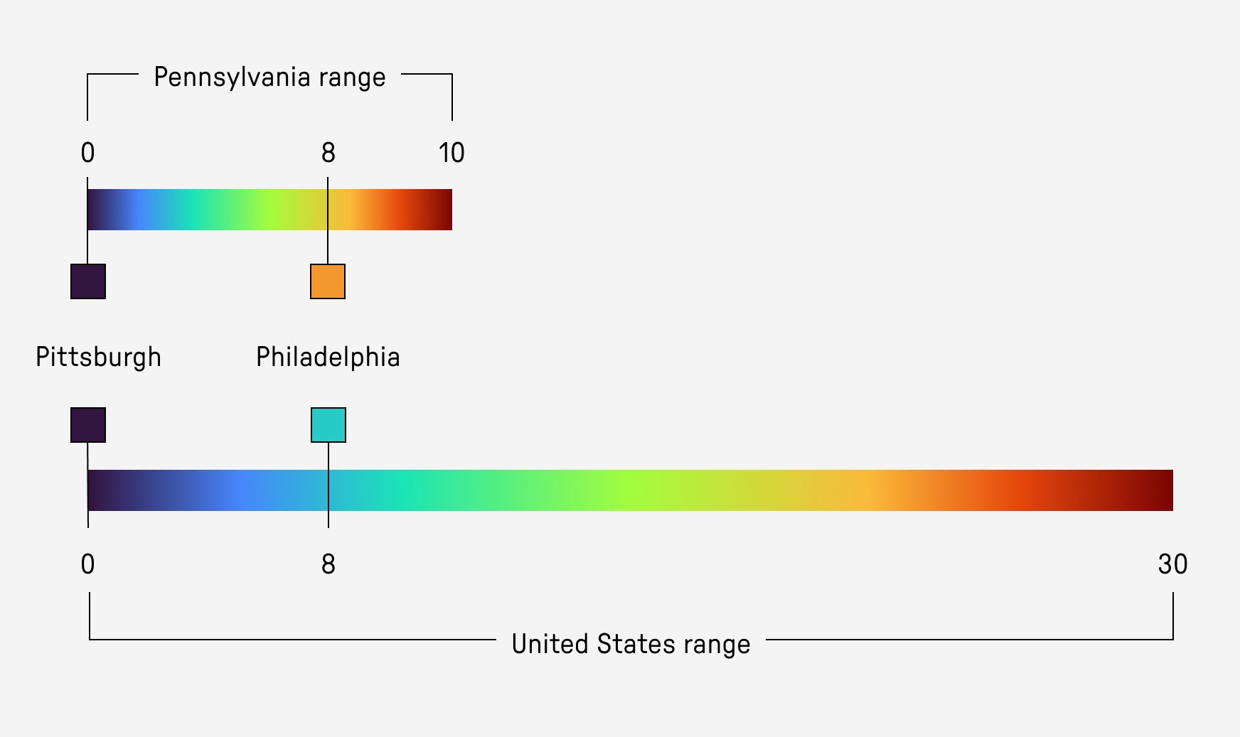
I think this is less of a problem when analyzing larger regions. Because there are such an enormous range of climates, the colorscale should reflect this. It’s more of an issue when the region is smaller and the relatively minor differences between climates are amplified.

Thoughts

While it was an enjoyable technical challenge, this experiment did not achieve what I wanted it to. I did quantify similarity in a broad climactic sense, but due to its generality it lost explanatory power. Which of the 60 metrics account for the differences? Where from place to place and month to month, where do the metrics diverge and where do they converge? Ultimately the original question is left unanswered: why do certain plants grown in a particular range? To what extent do climate variables predict that range?

I think answering these questions will be possible only at a smaller scale. It was the broadness and generality that led this experiment astray; the next try will be much more specific.

⁂